

Excel formulas: The most popular functions and tools, with examples - johnsondech1948
![]()
Plume Schultz
Stand out has over 475 formulas in its Functions Library, from simple mathematics to very complex applied mathematics, logical, and engineering tasks such As IF statements (one of our repeated favorite stories); AND, OR, NOT functions; Counting, AVERAGE, and MIN/MAX.
The primary functions covered below are among the most popular formulas in Excel—the ones everyone should have a go at it. To help you learn, we've too provided a spreadsheet with all the normal examples we cover below.
This spreadsheet contains a tab for to each one of the formulas smothered in this story, with example data. JD Sartain
1. TODAY/Forthwith
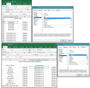
There are 24 Appointment and Time functions listed on the dribble-down menu under Formulas > Date &A; Prison term: 11 Date formats, 10 Time formats, and as many user-defined custom formats you can create. The TODAY subprogram reveals the rife calendar month, day, and year; while the NOW function reveals the current calendar month, day, year, and time of day. This is a handy function if you're one of those individuals who forever forgets up to now your exploit.
1. Enter the following formula in cell A1: =Now() and press Enter.
2. Succeeding, typewrite over that procedure in A1 with =NOW().
World-shattering NOTE: Why type over? In order for these two formulas to work properly, they must be entered in the Home cellular phone, that is, A1, other than, they won't update automatically when the spreadsheet recalculates. Press Change over- F9 to calculate/recalculate the athletic spreadsheet just, or press F9 for the entire workbook.
After you come in one of these functions in A1, you can then reformat the Date and Time surgery use the system default. The default format for the TODAY operate is 8/29/18, and the default option for NOW is 8/29/18 21:57. If these don't work for you, change them.
3. Position your cursor on the Date or Time you want changed and choose Home > Initialise > Format Cells.
4. In the Format Cells dialog window, prefer Date (or Clock time) from the Category panel subordinate the Number tab.
5. Scroll through the list of Engagement/Time formats in the Type dialogue pane and select the format that best fits your project.
 JD Sartain / IDG Worldwide
 2. Pith functions
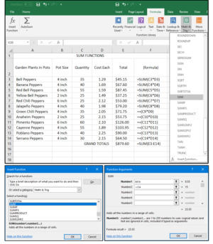
Probably the all but often used function in Excel (operating theatre any other spreadsheet program), =SUM does just that: It sums a column, course, operating theatre range of numbers—just it doesn't just sum. It too subtracts, multiplies, divides, and uses any of the compare operators to get back a result of 1 (trusty) or 0 (dishonorable).
You can also get the same results just exploitation the summation (+) sign in place of the function SUM. For example, both of these formulas produce the same answer: =SUM(J7*9) and =+(J7*9). In the spreadsheet graphic below, notice that cells E3 through E8 employ the SUM function, while cells E9 direct E9 through E14 economic consumption the plus (+) sign and the results are the same.
You can accede the SUM function (operating theater + sign in) manually or select it from the Decoration menu under Formulas > Math & Trig (button), then choose from the drop-down list; operating room choose (from the Ribbon menu) Formulas > Insert Function, so scroll down the list and select it from there.
If you just neediness to add a single column of numbers racket, position your cursor in the cell at the tail of that editorial, click the AutoSum button > SUM, and beseech Come in. Stand out frames the column of numbers in green borders and displays the convention in the current cellphone.
 JD Sartain / IDG Worldwide
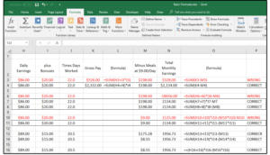
 The job comes when the range of numbers you motive to calculate gets complex with multiple calculation operators terminated multiple cellsFor object lesson: =SUM(H1+I1*J1-M1*J1. Remember your high schooling math? If the numbers racket inside the formula are not classified decently, the answer bequeath glucinium wrong. Notice the screenshot below (figure 2).
Enter upon the followers column headers in H2 through P2 (use EL+ Enter to stack headers in a only cell): Daily Earnings, Plus Bonuses, Times Days Worked, Gross Pay, (pattern), Minus Meals at $9.00 per day, Total Monthly Earnings, Normal, and Comment.
NOTE: The formula columns are FYI only and provide no intrinsic prize to the spreadsheet. They only "display" the recipe for your welfare (so you can see the syntax of apiece rule used).
For this exercise, you prat enter the same values in H3:11, I3:11, and J3:11, with or without the blank rows in 'tween (once more, added for easier viewing). Complete as follows: $86.00, $20.00, 22.0 workdays, and the rest are formulas. Preeminence that As we build for each one formula, we are combine the steps, eventually, into a single formula.
We depart with three separate formulas. The first is to add the Every day earnings, plus Bonuses, multiplied by the number of days worked in a calendar month, which equals Gross Pay: =SUM(H3+I3*J3) in electric cell K3. Acknowledge that the answer is $526.00. That fair-minded doesn't look right.
Use your calculating machine to check the formulas to ensure they're straight BEFORE you copy them to the take a breather of the cells in the column.
The formula in K3 is wrong. It requires group the numbers reported to the order of computation using commas or parentheses.
Note the corrected formula in cell K4: =SUM(H4+I4)*J4. See your numbers again (with your calculator) and take down that this formula is correct. The correct answer is $2,332.00.
5. The sec formula (in M4) is =SUM(J4*9) multiplies the workdays (22) times $9.00, the cost of meals per day. The correct answer is $198.00.
6. The 3rd formula (in N4) calculates the monthly earnings harmful the meals: =Heart and soul(K4-M4); answer is $2,134.00.
7. In the next group (H6:N8), the formulas in M6:M8 remain the same: =SUM(J7*9), etc.—over again that's the number of workdays times the cost of meals. But the formulas in column K are eliminated and so combined with the formulas in editorial M: =SUM(H7+I7)*J7-M7. Note that the phrase structure (the structure Oregon layout of the formula) is correct in cells N7 and N8, merely incorrect in N6.
8. The next mathematical group (H10:H11) combines the formulas in editorial M with the formulas in chromatography column N: =SUM(H11+I11)*J11-(M11*J11)—banker's bill that the formula in N10 is incorrect. By combining these formulas into one, you can eliminate columns K and L.
9. As wel, instead of "hardcoding" the price of the meals (as shown in M3:M4 and M6:M8), you stool like a sho change the terms of the meals in pillar M (M10:M11) when inflation dictates an growth alternatively of changing the rul.
 JD Sartain / IDG Worldwide
 3. RAND function
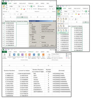
The RAND function is really simple and traditionally ill-used for applied math analysis, secret writing, gaming, gambling, and probability hypothesis, among gobs of other things. In Excel, the RAND function generates a random number between 0 and 1. Note; withal, that every metre you enter new information and press the Enter key, the list of random numbers you precisely created changes. If you need to maintain your haphazard numbers lists, you essential format the cells every bit values.
1. Enter the function =RAND() in columns A3 through with A14. Select that column and press Ctrl+C (for copy) or click the Copy push button under the Home tab and choose Written matter from the leave out-fallen menu. Move your cursor to cell B3 and blue-ribbon Home > Library paste > Spread Special. Click the Values button from the Library paste Extra dialog window, then click Oklahoma.
2. Now the listing contains values instead of functions, so it will not commute. Comment (in the formula bar) that the random numbers have 15 digits after the decimal (Stand out defaults to 9), which you can change, if necessary (as displayed in cell F3). Equitable detent the Increase Decimal clit in the Number group under the Home tab.
3. If you prefer to work with whole numbers, enter upon this formula in cell F3: =INT(RAND()*999) and you go a 3-digit random number. Copy the formula polish done F12, then hyperkinetic syndrome another '9' to the string to add other digit to your random number—e.g., four nines equal four digits, five nines equal five digits. Once again, you must copy the list and Paste as Values to keep down a static list.
 JD Sartain / IDG Worldwide
 4. COUNT functions
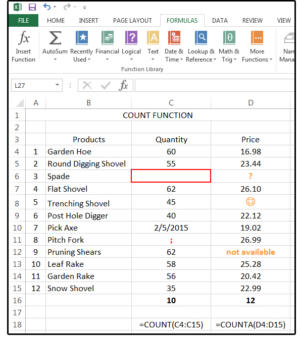
Use the COUNT function to count the add up of numeric values in a rove of cells; for instance: C4:C15 contains the quantity of garden tools Mr. McGregor inevitably to order for his shop. Note that the answer is 10 (out of 12), because the COUNT function does not include blank cells. However, if you enter a zero, a numeric codification, or a date, Excel counts it as an "occupied" cell and includes information technology in its response.
Enter 10 Numbers into pillar C (Quantity). Replace one number with a space (or a tapdance along the spacebar), then replace other number with a semicolon, and so enter a go steady into cell C7.
Get in this formula at the bottom of the amoun list (C16): =COUNT(C4:C15). The answer is 10 (out of 12) because Stand out counted all the numbers and the date, but ignored the blank cell (containing the distance) and the punctuation in jail cell C8.
Use the COUNTA function if you want to include numerical values, dianoetic or error values, textual matter, a space (from the spacebar), punctuation mark, symbols, or any other character along your keyboard.
1. Enter 12 dollar amounts into column D (Price). Replace one cell with a question commemorate, some other cellular telephone with a symbol, and another cell with close to text.
2. Participate this pattern in D16: =COUNTA(C4:C15). The answer is 12 (out of 12) because Excel included all the "non-numeric" values and characters.
3. Notice that row 18 (C and D) displays the actual formulas that are in C and D 16.
 JD Sartain / IDG Worldwide
 5. AVERAGE function
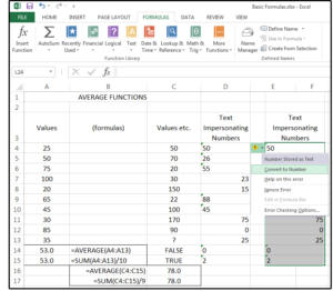
About everyone knows that an fair is dictated by adding all the values in a list, so dividing away the number of values listed; e.g., 4+5+3=12/3=4, which is the average. You can use the Marrow part and add up the division all in one formula, or you can just use the Ordinary function. The syntax is: =AVERAGE(place).
1. Enter some numbers in tower A. Enter the AVERAGE function at the bottom of the list: =AVERAGE(A4:A13) and note the suffice (in our case) is 53. You can verify your answer with the SUM part; that is: =SUM(A4:A13/10) = 53.
2. Next enter some many numbers in newspaper column C but, this time, ADHD around text to one cell, punctuation to some other, and a space to another. Enter the identical formula: =AVERAGE(A4:A15), and note the serve is 78. To affirm, enter the Marrow formula omitting the cells that contain non-numeric characters:
Cells that contain text, logical values, punctuation, or empty cells are disregarded; but cells with the zeros (Eastern Samoa a number, only non as text) are included. A text zero would have an apostrophe in front of the zero, which you cannot experience in the cell, merely is visible in the Chemical formula Bar.
IMPORTANT NOTE: If you're importing huge databases from a mainframe or an outside, external generator, sometimes the numbers export as text. How can you know if a number is really schoolbook? Generally, text is left-justified and numbers are right-even but, because everyone formats their spreadsheets for aesthetics directly, that method is unreliable. Other option is to scroll quickly through a long list of imported numbers and view the Formula Bar. If you see apostrophes before any of the numbers, those entries are text. Last, look for the green triangle in the top left wing street corner of the cell. Unless the previous owner of the spreadsheet instructed Excel to ignore this wrongdoing, then the contents of the cell are text.
If the values are text, you must convert them to numbers racket directly. To get along this, move down to the number 1 list in the list that's really textbook. Highlight the chain of text that's impersonating numbers. Exact-clink the yellow word of advice sign that's left of the first text cell in the range. Click Convert to Keep down from the pop-up list, and it's through with.
 JD Sartain / IDG Worldwide
 6. Fukkianese/Georgia home boy functions
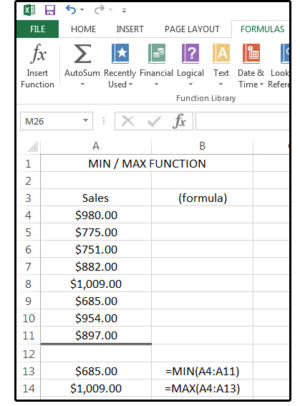
Use the MIN function to find the smallest number in a roll of values, and the MAX function to find the highest. The sentence structure for these functions are: =MIN(range); =MAX(stove) where range equals the list of numbers you'atomic number 75 calculative.
Unrefined uses of this function are; for example, find the highest/lowest grade in a classroom; the highest/worst gross revenue dollars in a store; the highest/last batten averages of your best-loved baseball team; etc..
Some would enquire, why not just sort the information? You could, just every time the numbers changed, you'd have to ray-sort. And, if you're categorisation multiple columns/fields with a lot of records/rows, the sort option could get cumbersome.
The MIN/MAX functions remain the equivalent heedless of the changes in the data, even if you bestow more rows (as long as you add the rows using the Insert > Wrangle feature within the existing wander—that is, higher up the cell that contains the rule).
Enter many numbers racket in column A4:A11, then enter this pattern in A13: =MIN(A4:A11) and this formula in A14: =MAX(A4:A11).
NOTE: The MIN/MAX functions disregard empty cells, TRUE/FALSE answers, textual matter, text impersonating numbers, symbols, and punctuation.
Next dormie, the powerful Concatenate function that combines denary cells' Charles Frederick Worth of data! Keep reading for more great formulas.
 JD Sartain / IDG Worldwide
 7. CONCAT/CONCATENATE
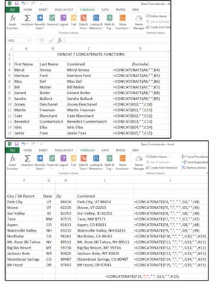
The functions CONCAT and CONCATENATE do the Same thing: They both combine multiple cells, ranges, operating room strings of data into one cell. The most common use of this function is to combine above all discover into one cell OR join the city, state, and ZIP code into one cell.
Annotation: CONCAT replaced CONCATENATE in Excel 2016, but some functions are still available. Observe that CONCAT appears only under Formulas > Text and Formulas > Insert Function > Category > Text edition, but both CONCAT and CONCATENATE appear under Formulas > Stick in Function > Family > Every last.
Enter whatever first names in editorial A and cobbler's last names in column B. Enter the following formula in column C: =CONCATENATE(A4," ",B4) or =CONCAT(B4," ",C4), then copy the formula down. What are the threefold quotes for? Run into Note below #2.
2. Enter a a couple of cities (or ski resorts) in editorial F, states in column G, and ZIP codes in column H. Embark the following expression in column I: =CONCATENATE(F4, ",", " ", G4," ",H4).
Notice: If you want a space between the first and conclusion describ, you must put down that space inside quotation marks in your formula. The same matter is true for punctuation, such as a comma between city and state. In the following formula the "," (quote comma quote—in red) tells Stand out to insert a comma between the data in F15 (city) and the data in G15 (state). The " " (quote blank quote—in purple) adds a space subsequently the comma butterfly betwixt F15 (city) and G15 (state) and some other distance 'tween G15 (state) and H15 (zip code).
=CONCATENATE(F15, ",", " ", G15, " ",H15).
 JD Sartain / IDG Worldwide
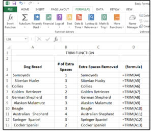
 8. TRIM
This function removes surplus (operating theater padded) spaces that taint your data every bit a result of user error, downloading information from an foreign source such as the Net, OR importing data from another computer system. And you don't own to "tell Excel" where the spaces are located in the string of text in to each one cell; it recognizes the extra spaces and removes them. Note; however, that IT will not remove a space in the midst of a word. The syntax is simple: =TRIM(cubicle address).
1. Enter around information in column A. Add some spaces in front, after, and in the midsection of multiple run-in, then enter the following formula in cell A4: =TRIM(A4).
2. Copy the rul Down. It's that unchaste!
Annotation: In that location is single sheath where this function does not work, and that's with a non-breaking space graphic symbol used in webpages. The decimal appreciate is 160, and the HTML write in code is  . You can remove this character using a combination of Tailored, CLEAN, and SUBSTITUTE.
 JD Sartain / IDG Worldwide
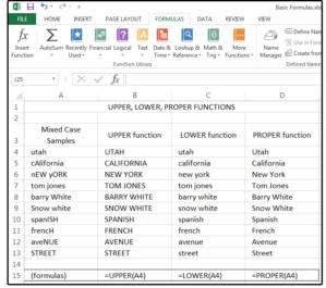
 9. Pep pill/Lower berth/PROPER
Another easy group, these functions convert text in a cell operating room set out of cells to uppercase, small letter or proper pillowcase. Proper case is introductory alphabetic character in caps and remaining letters in lowercase. The syntax is wide-eyed: office, cell direct.
1. Enter some intermingled-case data in column A; e.g., California, nEW York, spanISH. Enter the following formula in column B: =Amphetamine(A4), in pillar C: =Get down(A4), and chromatography column D: =PROPER(A4).
2. Notice that Excel corrects all the misplaced example errors and converts the information correctly. Copy the formulas down, and that's it for this simple one.
NOTE: In Word, you can use Work shift-F3 to cycle through great, minuscular, and priggish case, simply this cutoff key is not available in Stand out. Take down that the Excel function =PROPER is called Sentence showcase in Give-and-take.
 JD Sartain / IDG Worldwide
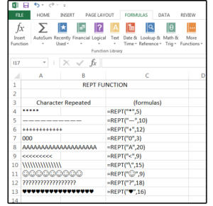
 10. REPT
When White lotus 1-2-3 was the only game in town, you could embark a backslash followed by some character and Lotus would recapitulate that character passim a cell. If the cell width grew larger or smaller, so did the character. In Stand out, this feature is handled by the function REPT. It's not quite equally prompt because you mustiness add the character to the formula, then specify how many times you want that grapheme repeated. This means if the cell width is increased, the repeated character is not, and if the cell width is decreased, the repeated character bleeds over into the adjacent cell.
The syntax for this function: =REPT("*",5); =REPT("—",10), =REPT("+",12). You can double whatever fictional character on the keyboard plus symbols.
 JD Sartain / IDG Worldwide
 11. IF instruction
The IF function (also more commonly called IF statements) work like this: IF, then, else. In essence, that means if a condition is true, then do one thing, else/otherwise answer something else. For representative, if the puppy is a Labrador, then purchase a blue collar, otherwise/other, buy a red nail.
The syntax (the way the commands are organized in the formula) of the IF assertion is: =IF(logic_test, value_if true, value_if_false). IF statements are used in completely programming languages and, although the sentence structure may alter slightly, this operate provides the duplicate results.
1. Enter the followers column headers: Cookie Boxes Sold; 3rd Choice =More than 500 Sold, Less than 1000; 2nd Prize =More than 1000 Sold-out, Less than 1500; 1st Prize =More than 1500 Sold, Less than 2000; Grand Prime =More 2000 Sold
2. Introduce some numbers into column A4:A13. Integrate IT high so you get data all told of the Sold columns.
3. Enter this pattern in B4: =IF($A4>500, $A4, 0).
NOTE the $ signboard in front the column letter 'A' in the above formula. Invest your cursor on the first 'A' in the formula, then use the use key F4 to cycle through the Utter and Relative References. Stop when the $ sign of the zodiac precedes the 'A' (for for each one A in the formula). This tells Excel NOT to shift the column letter, merely only change the rowing Numbers when this convention is copied. If you put a dollar sign ahead some the column letter and the quarrel add up, neither would change.
4. Copy the formula in B4 to C4, D4, and E4, then edit As follows: C4 =IF($A4>1000, $A4, 0); D4 =IF($A4>1500, $A4, 0); and E4 =IF($A4>2000, $A4, 0). Then written matter down.
5. The expression works, but you have to retrospect each column to see who North Korean won the prizes, because each column shows Altogether the values greater than the amount in the formula. That's all right for a small spreadsheet, but not for anything bigger than a single screen.
6. We need a Nested IF statement for this one. Repeat numbers game 1, 2, and 3 above start on row 20; but rather of the formula in 3 above, enter this rule in B20: =IF(AND($A20>500,$A20<1000),$A20,0).
7. Repeat act 4 above, but redact the formulas like this: C20 = =IF(AND($A20>1000,$A20<1500),$A20,0); D20 = =IF(AND($A20>1500,$A20<2000),$A20,0); and E20 = =IF($A20>2000, $A20, 0). Yes, this last one is different because thither is atomic number 102 "less than" amount. And then imitate downbound. Now you can reckon at to each one column and determine immediately who the winner is for that category.
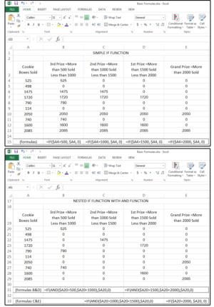 JD Sartain / IDG WorldwideBasic IFstatements and nested IF statements
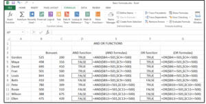
 12. AND/OR
AND and OR are common functions in the programmers' environment, also referred to as Boolean operators (along with Non). AND way that all conditions in the question essential be true; OR substance that at least one shape must comprise true.
For example, superficial for an applicant with MS Word AND MS Excel experience way the applicant mustiness cause both skills to qualify for the job. This condition would provide a TRUE termination. Looking an applicant with MS Word Operating theater Surpass means the applier essential have one OR the other, but not necessarily both. Also a TRUE result. Having neither skills would, obviously, provide a FALSE result.
1. Copy the numbers from the spreadsheet in figure 13, operating theater download the full workbook (link down the stairs).
2. Go in the following AND formula in cubicle D4: =AND($B4>=501,$C4<=500). Again, note the $ signs. Then copy down to cell D13.
3. Enter this formula in cell F4: =Oregon($B4>=501,$C4<=500), then simulate down. Detect the results in the rows with borders; that is, 5, 8, and 13. The AND results are all FALSE because both conditions were false (or not actual); while the OR results were complete TRUE because one of the conditions was true, patc the other was false.
If this seems puzzling, study the numbers in columns B and C. Then read the formulas that calculate for the AND function, then the OR function, and it will make more sensation.
 JD Sartain / IDG International
 13. NOT
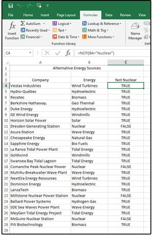
Having explained preceding how the AND and OR functions (also known as Boolean operators) work, the third Mathematician operator in that mix is the NOT function. Ever search through a really long list of data and wish you could remove each the entries that do NOT apply? For example, I want to see everything available about choice energy EXCEPT (or NOT) nuclear.
In Excel, it's an easy task. Make over a leaning of 25 companies that provide various alternative get-up-and-go sources and what those resources are (columns A, B, C; begin on row 4). Enter the following formula in cell C4: =Non(B4="Atomic"). Then copy the convention from C4 down to C5:C28.
If the response is TRUE, the energy reference is Non nuclear. If the response is Treasonably, the energy source IS nuclear. Yes, information technology's reverse logic and you whitethorn not instantly see a need for this function but, if you'atomic number 75 an wishful Excel user, you will find out many reasons to use this formula in the approaching.
TIP: Remember that Boolean logical system applies throughout all database programs, including your favored hunting engines. The Boolean operators AND and OR must be in all-caps to serve as an operator. In Google, the Boolean Non operator is the minus sign; for example, to list all alternative energy sources EXCEPT nuclear, typecast this in the research field box: list all disjunctive energy sources –nuclear.
Got text edition and numbers with delimiters all finished the place? Keep meter reading for the formula to deposit that.
 JD Sartain/IDG
 Using the NOT Boolean operator
14. RIGHT & Text-to-Columns
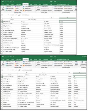
Imagine that your boss just transmitted you a single file with 100,000 names and addresses compiled from several data dumps off multiple different database systems, such as Oracle RDBMS, SAP Sybase ASE, Informix, MongoDB, Redis, and Couchbase. The file is in a CSV (Polygonia comma separated values) delimited format, thusly you can open it in Excel, merely the delimiters are terminated the place—some are commas, some are spaces, just about are tabs, etcetera. Your chore is to reformat the run-on data into five fields: Name, Address1, Address2, City, and State.
A. First, separate the city, country, and ZIP codes into different columns. Select column C (City, State, Zipp), then pick out Information > Text to Columns. Assure the Delimited button is checked, then chatter Next. On the next projection screen, ensure that the Comma box is checked, then detent Next. Browse direct the list to insure the separation is correct, past click Ending. Stand out divides the extraordinary column into two.
B. Now we need to separate the ZIP codes from the submit names. For this task, the Text to Columns option would not be accurate, because the only delimiter available is a space. Because close to of the states have multiple names such as Prince Edward Island, the Text edition to Columns function would spread the data across too many columns.
C. The solution is to use the =RIGHT function. Because more or less of the ZIP codes have five digits and some have 6, enter the following command in cell E2: =RIGHT(D2,6), so copy from E2 down to E3 through E16. Finished. Column E now contains ZIP codes only. However, editorial D hush has both states and ZIP codes.
15 & 16. LEFT & LEN
Use this function to segregated USA from the ZIP codes. Enter the next normal in cell F2: =LEFT(D2,LEN(D2)-6), then copy down from F2 to F3 through F16. Basically this formula says pass away to cell D2, count 6 places from the left and remove those characters, departure the remaining characters in cell D2 (regardless of how many). As long as one piece of information inside a cell is alone, you can exercise that entropy to add, edit, or supervene upon other data inside that cell.
To move or pull strings the data in columns E OR F (which take formulas), highlight the tower and choose Copy, prompt cursor to another column, and choose Spread Special> Values, so click OK.
 JD Sartain/IDG
 Using the The right way, LEFT, and LEN functions
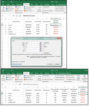
17. PMT
Use this handy function to determine how so much your payments would get on that new car you just took for a test drive. The process is simple: Enter the procedure followed by the interest rate divided past 12 (for 12 months), the Term (or number of monthly payments), followed away the Loan Amount.
Embark this recipe in cell F2: =PMT(D2/12,E2,C2,0,0), then re-create from F2 down to F3 through F6.
To calculate a down payment, enter the down payment percentage in column F; move into the formula in column G; enter the adjusted loanword amount formula in column H; and the new time unit payment formula in tower I. Also, change the Term (in months) to Term (in years) in column E—e.g., instead of 360 months for the House Loan, enter 30 eld.
Enter the following formula in cell G10: =SUM(C10*F10). Enter this formula in cell H10: =SUM(C10-G10). And enter this chemical formula in cadre I10: =PMT(D10/12,E10*12,H10,0,0). Observe that the Rate of interest is still divided by 12, and also, that the Term (in years) is multiplied by 12.
 JD Sartain/IDG
 Use the PMT function to calculate your auto payments for that new car
Handy tip: Ever so wonder wherefore or s currency formats heart the dollar number and the dollar mark sign ($1500.00), while others push the numbers aligned to the right and force out the dollar mark allied to the left-hand ($ 1500.00)? To center the number and dollar mark, highlight the cell, and choose Base tab > Number group > Number Formatting > Currency. To align the dollar left-wing and the numbers right, highlight the cell, then click the $ symbolization in the Number group.
Note: When you purchase something afterward clicking links in our articles, we may take in a small commission. Show our consort connectedness policy for more details.
JD Sartain is a technology journalist from Boston. She writes for PCWorld, Electronic network World, CIO, & several other tech magazines.
Source: https://www.pcworld.com/article/402534/excels-top-12-most-popular-formulas-with-examples.html
Posted by: johnsondech1948.blogspot.com
0 Response to "Excel formulas: The most popular functions and tools, with examples - johnsondech1948"
Post a Comment